GUI tutorial
To start the GUI, either execute this command in a terminal:
python -m deepcinac
Or execute the python code:
deepcinac.gui.cinac_gui.launch_gui()
If you don’t have data, we provide a demo dataset with a calcium imaging movie, ROIs (cell coordinates) extracted by Suite2P (this file and this one) and the predictions from our general classifier.
First window: data to display
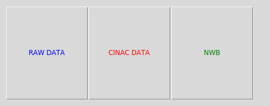
The button RAW data allows you to load data that haven’t been processed using the GUI previously (see below).
The button CINAC data allows you to load data that have been processed using the GUI.
The button NWB data allows to load calcium imaging contained in a Neurodata Without Borders (NWB) file. For the option to be available, you need to install the package pynwb. You can also use nwb to launch predictions using our toolbox CICADA.
Raw data parameters
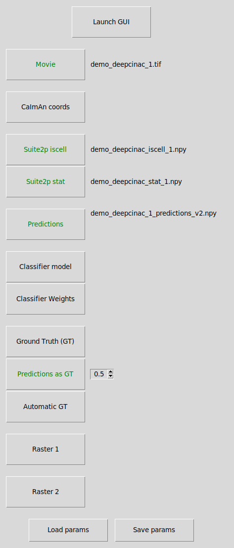
This window will allow you to choose which data you want to display in the GUI.
When you select a file in the .npz or .mat format, a menu will appear letting you choose which attributes of the file should be loaded.
We will describe the function of each button below:
Launch GUI: launch the exploratory GUI, the button will be enabled when you have selected a movie file and some ROIs.
Load params: Select a .yaml file that contains the parameters to be load.
Save params: Allow to save in a .yaml file the parameters that have been selected in this window, to be loaded later.
Movie: Select the calcium imaging movie file, so far only tiff format is supported.
CaImAn coords: Select the file containing the CaImAn cell coordinates (ROIs). It can be a file in numpy (.npy or .npz) or matlab format (.mat). If the coordinates have been computed with matlab, meaning the indexing starts at 1, check the box “matlab indexing”. CaImAn coordinates as we used them are represented by a list (if 2d-array) of 2 lines representing x and y coordinates of the contours’s points.
Suite2p iscell: Select the file iscell produced by suite2p indicating which cell is valid.
Suite2p stat: Select the file stat produced by suite2p containing the cell’s pixels
You can either load coordinates from CaImAn or from Suite2p but not both.
Predictions: Select a file containing the predictions from the classifier. It contains a 2d array of n_cells * n_frames with float values between 0 and 1. By loading this file, you will be able to display the predictions in the GUI. You would also be allowed to click on the button “Predictions as GT” to used those predictions with a specific threshold to fill the GUI with this ground truth as a base.
Classifier model: Instead of loading predictions, you can load the model (.json file)
Classifier Weights: and the classifier weights (.h5 file). This will allow you to run the classifier cell by cell and display the predictions on the GUI. If you haven’t configured your GPU and use the CPU, it might take a few minutes to predict the activity for each cell depending on how long is your recording.
By clicking one of the 3 following buttons, the GUI will display peaks and onsets determined by one of this button. Otherwise, by default, the fluorescence signal will be displayed without any peaks and onsets. You’ll be able to add some. If some are loaded, you will still be able to modify them.
Ground Truth (GT): Select a file that contains a 2d array of dimension n_cells * n_frames, it should be a binary matrix, containing only 0 and 1, 1 indicating that a cell is active at a given frame.
Predictions as GT: If a predictions file is loaded, you can set the threshold that will be used to decide the periods of activity of the cells and onsets/peaks according to those transients.
Automatic GT: Based on the smooth version of the fluorescence signal, all potential onsets and peaks will be added.
Raster 1: Select a file that contains a 2d array of dimension n_cells * n_frames, for each value > 0, a line will be displayed at the bottom of the fluorescence signal section (the matrix is binarized), thus representing the activity of the cell (either as a spike inference or representing transients like CINAC). It allows the comparison of the results of the predictions or your own ground truth with another method. It is displayed in green.
Raster 2: Same as raster 1, but allows you to add one more raster.It is displayed in blue.
Cell type config: Mandatory to display the predictions. It should be the same yaml file than the one used to train the cell type classifier. The file indicates which cell type are the output of the classifier. You can find examples here.
Cell type predictions: Select a file containing the predictions from the classifier. It contains a 1d array representing the indices of the cells predicted and a 2d array of n cell types x n_cells with float values between 0 and 1. By loading this file, you will be able to display the predictions in the GUI.
Cell type model: If the predictions don’t cover all the cells, you can load the model (.json file)
Cell type weights: and the classifier weights (.h5 file). This will allow you to run the classifier for any given cell and display the predictions on the GUI. If you haven’t configured your GPU and use the CPU, it might take a few minutes to predict the cell type.
CINAC data parameters
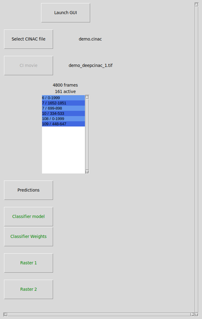
This window will allow you to choose which data you want to display in the GUI.
The cinac file (extension .cinac) is the format used to save ground truth data produced using the GUI.
We will describe the function of each button below:
Launch GUI: launch the exploratory GUI, the button will be enabled when you have selected a cinac file.
Select CINAC file: Select the cinac file to open.
CI movie: this button will be enabled if no movie file reference is contained in the CINAC file or if this reference doesn’t match an existing file. Thus allowing you to select the calcium imaging movie that matches the cinac file. The calcium imaging movie should be the original one used to produce the CINAC file that matches the cell contours contained in the CINAC file. Moreover, selecting a CI movie is not mandatory to open a CINAC file, if no movie is indicated, then segments will be opened separately (see below).
Listbox: displays the segments for which a ground truth has been made. Each line of the listbox represents a segment, with the given format “{cell} / {first_frame}-{last_frame}” the cell the segment is from and the frames it contains. If no CI movie is available, then you need to select the segment you want to display. A distinct window will be opened for each segment, up to 10 can be opened simultaneously. In that case, only the pixels surrounding the cell will be displayed in the GUI, the number of cells available will correspond to the number of cells that overlaps with the cell of the segment. In that mode, no modification of the segment can be saved, it is necessary to have the original movie to make modifications. On top of the listbox, it is displayed the number of frames that are comprised in the segment as well the number of active frames, meaning frames that are contained between an onset and a peak (corresponding to the transient rise time)
others buttons: same usage as the ones in the window “Raw data parameters” (see above). However, those buttons will be enabled only if a CI movie is available.
NWB data parameters
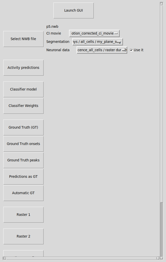
This window will allow you to select the content from a Neurodata Without Borders (NWB) file you want to display.
We will describe the function of each button below:
Launch GUI: launch the exploratory GUI, the button will be enabled when you have selected a NWB file.
Select CINAC file: Select the NWB file to open. The NWB file should contain at least one (two photon) calcium imaging movie and some data regarding segmentation (as ‘pixel_mask’). If neuronal data ara available, they will be displayed.
others buttons: same usage as the ones in the window “Raw data parameters” (see above).
Exploratory GUI
The exploratory GUI has two main goals:
to visually evaluate inferred neuronal activity from inference methods
to build a eye inspection-based ground truth
In order to build a ground truth, you need to annotate the data either adding onsets/peaks for neuronal activity or indicating the cell type. For each cell, you can save any segment (of continuous frames) of data. The annotated data will be saved in the format of .cinac files.
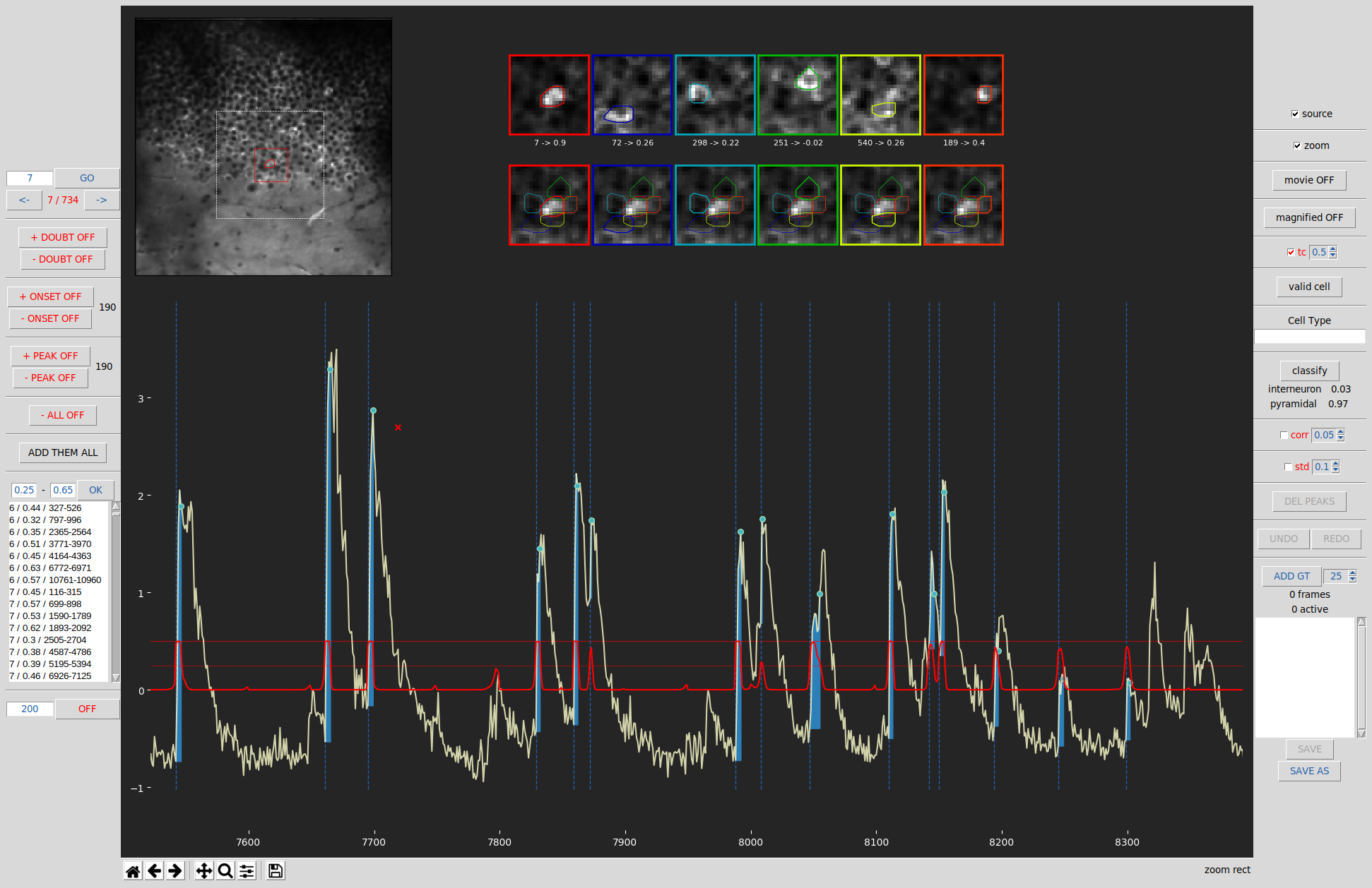
Central Panel:
Average movie view: When the movie is not being played, on the top left is displayed the average of all movie’s frames. The cell currently viewed is represented on the map by a red contour. You can click on any cell to set the selection to this cell. The dashed white edge square represents the view displayed when playing the movie in the zoom mode. The red edge square represents the pixels that will be saved and used for the current cell by the classifier.
Movie player: On top left, when the movie is being played (by clicking on the first and last frame to be played after activating the movie mode). On top-left corner the current frame number is displayed. The current cell has a red edge contour. Finally, the fluorescence signal of the current cell is displayed (the red part represents the frames already played and the white part, the ones coming).
Source and transient profiles: displayed on the top right if source mode has been activated and a transient has been selected. The top row represents the source profile of the cells (the current one, always on the left side, and the ones overlapping it). Source profile represents the weighted average pixels intensities of the cell during the rise time of its highest transients. On the bottow row is displayed the transient profiles that represents the weighted average pixels intensities of the cell during a given transient (the one before or at the red cross). Finally, between those 2 rows are displayed for each cell, its number and the Pearson correlation between the source profile and transient profile (for the pixels contains in the ROIs of the cell).
Magnifier: displayed on the top right when the magnifier mode is on and the onsets/peaks mode are one. It allows to displayed a zoom version of the fluorescence signal displayed belown thus allowing a more precise annotation of the signal.
Fluorescence signal: on the bottom, the average fluorescence signal (z-score normalization) of the current cell is displayed. The blue dashed vertical line represents the onsets. The blue dots represent the peaks. If the predictions mode is on, then a red line will represent the predictions of the classifier for this cell (see the right panel section bellow for more details). A black vertical span might be displayed to represent the a doubtful segment.
Navigation toolbar: displayed on the bottom, under the fluorescence signal window. The home button allows to come back to full signal view. The left/right arrows allow to come back to the last part of the signal visualized. The 4 way arrows allows to move the signal displayed. The magnifier button allows to zoom on one portion of the signal. The floppy button allows to save the signal plot as an image. Note that this is the toolbar provide by matplotlib and tkinter, however we notice that sometimes the buttons are not reactive, in that case the trick is to click on the plot then back to the button a few time until it does work again. We will rewrite the toolbar in a further version.
Left Panel:
Cells selection: the text field allows to write the cell number you which to display. Then press the enter button or click on the OK button. You can also use the arrows button to display the previous/next cell. You can also use shortcuts ctrl-left/right arrow to display the previous/next cell. Finally, you can also click directly on the cell you want to display in the cells map
DOUBT buttons: add or remove segment of doubt. Doubt segments are sections that should not be used for training the classifier as ground truth is difficult to establish. Just click on the start and end of the segment on the fluorescence signal section.
+ onset button: activate/deactivate the add onset mode. Allows you to add onset, just click where you want to add an onset. A dashed blue vertical line will appear at that position. Next to the button is displayed the number of onsets for this cell.
- onset button: activate/deactivate the remove onset mode. Allows you to remove onset(s), click 2 times with the mouse on the “fluorescence signal” part to indicate the start and the end of the movie segment from which you want to remove onsets.
+ peak button: activate/deactivate the add peak mode. Allows you to add peak, just click where you want to add an peak. A blue dot will appear at that position. Next to the button is displayed the number of peaks for this cell.
- peak button: activate/deactivate the remove peak mode. Allows you to remove peak(s), click 2 times with the mouse on the “fluorescence signal” part to indicate the start and the end of the movie segment from which you want to remove peaks.
- ALL button: activate/deactivate the remove all mode. Allows you to remove onset(s) and peak(s), click 2 times with the mouse on the “fluorescence signal” part to indicate the start and the end of the movie segment from which you want to remove onsets and peaks.
Add them all button: when clicked, it will remove all onsets/peaks present in the current window displayed and add all potential onsets/peaks that can be found using the change of derivative sign from a smooth version of the fluorescence signal.
Predictions listbox: this listbox is displayed if either predictions results are available or if a model and weights files have been selected. The listbox display the transients of the cells according to their predictions score. The text fields above it, allow to change the value boundaries of the predictions displayed. When clicking on a line of the listbox, it displays the given transient, that will be centered on the window, the number of frames on the window will correspond to the number displayed on the text field below the listbox. Finally, you can either double-click on a given transient in the listbox / push the ADD GT button / or press the G keyboard touch to add the given window the ground truth segment list.
Center Segment mode: you can change the size of the segment used when a frame is centered over the window displayed. By clicking on the OFF button, you active the center segment mode, then you can click on the “fluorescence signal” section, and the frame you click on will be then at the center of the window, the window number of frames will then be the one indicated on the text field.
Right Panel:
Cell / Neuropil / Cell - Neuropil checkboxes: allows to choose which trace(s) you want to display. ‘cell’ displays the raw signal (z-score normalization), Neuropil displays the neuropil surrounding the cell, and ‘Cell - Neuropil’ displays the raw signal substracted by the Neuropil one.
Source checkbox: activate the source mode (shortcut keyboard: s touch). Then to display the cells sources and transient, you need to click in the transient you want to display or just after. However, the transient need to be identified by an onset and a peak, if none exists you must add it before you can display the transient profile.
zoom checkbox: activate/deactivate the zoom mode. When on, a white dashed square will be displayed on the average calcium imaging movie view. The square represents the view displayed when playing the movie in the zoom mode.
movie button: allows you to play or stop the movie. (shortcut keyboard: space bar). To play it, click 2 times with the mouse on the “fluorescence signal” part to indicate the start and the end of the movie segment you want to play. To stop the movie, either press the space bar or the button “movie ON”. The movie will repeat until you do one of these actions. You might encounter some memory issues if you let it loop too many times.
Magnified button: Activate/deactivate magnifier mode. Will only appear if the onset or peak mode is active. Allows the display a zoom mode of the fluorescence trace on the upper right section of the GUI, thus allowing to be more precise without having to zoom on the main section.
tc checkbox: To display predictions. Click on it and either the predictions will be immediately displayed if you have pre-loaded them or it will be predicted using the model weights you have provided. A bold red line will then be displayed representing the prediction value, between 0 and 1. The 0 is labeled in the y-axis. The 0.5 is represented by the dashed red-line, the 1 by the top thin solid line. The interior of the fluorescence signal will be fill with blue when the prediction passes the threshold. You can set the threshold using the spin box next to the checkbox (Default value is 0.5). The checkbox is not displayed if no predictions or model/weights files have been selected.
valid cell button: identify the cell as valid (by default) or invalid.
cell type field: allows to indicate the cell type of the cell. It will be saved in the cinac file if you save any segment of the cell.
classify button: will be display only if a model and weights files have been provided. Run the classifier on the current cell, and display below the predictions score for each cell type as determined in the cell type yaml file given. If the predictions are loaded, they will be directly displayed.
corr: similar to std checkbox below, but set a threshold of correlation between the transients profile and the source profile of the cell. It can take a bit of time to compute depending how many peaks and onsets are present. The transient under the threshold will be displayed in red (if other correlations with overlapping cell are also low), and can be deleted using the “DEL PEAK” button.
std checkbox: set a threshold. All peaks (from smooth trace) that will be under the threshold will be colored in red. Then using the “DEL PEAKS” button, they will be deleted with their associated onsets. It can be useful when you use automatic onsets & peaks initiation and just want to eliminate the obvious noise.
DEL PEAKS button: allows to delete the peaks selected using the corr or std checkbox
UNDO & REDO buttons: to UNDO & REDO actions.
Ground truth segment: section that allows to select ground truth segment that will be used to train a classifier. The spinbox next to the “ADD GT” button allows to change the size (in pixels) on the square surrounding the cell and that represent the content that will given to the classifier. The “ADD GT” button allows to add the current cell and window displayed (frames displayed in the fluorescence signal section) as a ground truth segment, a new line will be added in the listbox. You can click on the line in the listbox to display the segment. To remove a segment, double click on it.
shortcuts:
Space bar: allows you to play the movie. Same effect as clicking on the button “movie OFF”. Then click 2 times with the mouse on the “fluorescence signal” part to indicate the start and the end of the movie segment you want to play. To stop the movie, either press the space bar or the button “movie ON”. The movie will repeat until you do one of these actions. You might encounter some memory issues if you let it loop too many times.
s: activate the source mode, same effect as clicking on the source checkbox. Then to display the cells sources and transient, you need to click in the transient you want to display or just after. However, the transient need to be identified by an onset and a peak, if none exists you must add it before you can display the transient profile.
o, O: activate/deactivate the onset mode. Allows you to add onset, just click where you want to add an onset. A dashed blue vertical line will appear at that position.
p, P: activate/deactivate the peak mode. Allows you to add onset, just click where you want to add a peak. A blue dot will appear at that position.
r, R: remove mode, will remove all onsets or peaks that are present between your first click and second click on the fluorescence signal section.
ctrl + left or right arrow: Switch to previous or next cell display. You can also indicate the cell to display in the text field. Another option, is to directly click on the average calcium imaging picture to select the cell you want to display.
left or right arrow: if you are zoomed on the fluorescence signal, then it will shift to the previous or following frames.
a, A: same effect as left arrow
q, Q: same effect as right arrow
m: magnifier mode. Will only appear if the onset or peak mode is active. Allows the display a zoom mode of the fluorescence trace on the upper right section of the GUI, thus allowing to be more precise without having to zoom on the main section.
c, C: activate/deactivate the center segment mode. If activated, center the window to the frame that will be clicked after pressing this touch. The size of the new window will correspond to the number of frames indicated in the text field under the listbox on the left panel. It allows to make sure the event you labeled will at the centered of the window, thus allowing a bigger representation when temporal overlaps before using it to train the classifier.
z, Z: activate/deactivate the zoom mode. When on, a white dashed square will be displayed on the average calcium imaging movie view. The square represents the view displayed when playing the movie in the zoom mode.
g, G: allows to add the current cell and window displayed as a ground truth segment.
T: if cell type predictions are loaded, then it allows to display the next cell (in indices order) with the same cell type as the cell currently display.